One of the challenges hardware (and software) manufacturers are facing is estimating the future level of support required in maintaining their products. Underestimating the support requirements would lead to major loses on the support contract while overestimating hurts the competitive edge of the product.
Future level of support includes: replacements, repairs, remote and on-site support. To that end, manufacturers develop reliability models for everything from hard/flash drives to cars and aircraft. These models take into account different configuration parameters of the final product and its internal components.

In 2007, Google conducted a large-scale analysis for a subset of its drive population. It utilized an environment containing a large number of disk drives, collected different types of data from these drives to a Big Data store (Google’s Bigtable) and conducted an analysis of the different Key Performance Indicators (KPIs) and their correlation with drive mortality:
- Manufacturer, Models and Vintage
- Temperature
- Utilization
- Self-Monitoring, Analysis and Reporting Technology (S.M.A.R.T)
Contrary to expectations, Google’s researchers found that these KPIs are more useful for predicting trends for a large population than for predicting a single drive failure.
Such studies help assess product reliability and the required amount of expected support for a product coming out of the assembly.
In many cases, an assembly line is used to create multiple copies of the exact product from exactly the same components (as in the case of hard drives belonging to the same series and lot). This makes reliability modeling and support estimation relatively straightforward. In other cases, as with EMC enterprise grade products manufacturing, products may be manufactured in a variety of very different configurations using an assortment of different components.
Support Level Quantization in EMC
EMC provides custom solutions to our customers, tailoring the best storage, virtualization, cloud and security solutions to enable flexibility in choice and dynamically configured environments. In light of this guiding principle, it should not be surprising to find that one of EMC’s enterprise flagship products has a very large number of possible configurations. One executive once said that, “no two enterprise grade products are created alike and being used in exactly the same way, under the same conditions”.
In this setting and as the reliability of the product is always the first consideration (which means, amongst others, redundancy of components), how do we now forecast the level of support required for each of these custom tailored products?
To answer this challenge, in a Big Data analytics project led by EMC Global Services

(Read Global Service InFocus Blog), we developed the Population Based Ranking (PBR) model for support quantization. This model clusters the different product configurations into small groups of similar makeup.
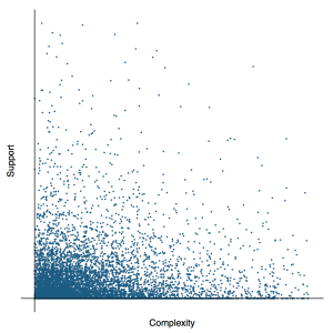
The support requirements are then modeled using regression analysis. The result is visualized as “Support Cost” compared to “Complexity”. This allows EMC Global Services to easily identify abnormal service costs of specific items. [figure 1]
How was this accomplished?
Let me explain in detail. We initially identified several KPIs that are highly correlated with the required level of support. We then introduced these KPIs as features to a machine-learning algorithm that constructs a baseline estimator for support requirements from the entire population. The following process is conducted on a week-by-week basis:Identify products deployed at customer sites that roughly share similar configuration details
1. Identify products deployed at customer sites that roughly share similar configuration details
2. Formulate a regression model that represents a baseline of similar sub-populations. An example of such a regression model is the Linear Regression model: where the optimization objective is to find the set of parameters that represents a ‘best fit’ of model to the data. [equation 1 below]

3. One such optimization criteria may be the Mean Squared Error (MSE): [equation 2 below]

4. Quantize the distance of actual support vs. the expected support calculated by the model for each of the items
For data storage, querying and analytics we utilize a Pivotal Greenplum database sandbox provisioned to Global Services by EMC IT’s Business Analytics as a Service. As the modeling process requires fitting a regression model to the entire population on a week-by-week basis, we make use of the MADlib machine learning library that provides Big Data machine learning capabilities in SQL. The API for regression analysis in MADlib enables fitting a model to a grouped set of data points, which matched our requirements perfectly:
The output from this modeling process, when projected to one of the KPI dimensions for one of the weeks analyzed looks like Figure 1:
Colors are ranging from green (0 – very low level of effort compared to peers) to red (8 – high level of effort compared to peers).
- Colors are ranging from green (0 – very low level of effort compared to peers) to red (8 – high level of effort compared to peers).
- The X-axis represents the complexity of the assembly for each item and the Y-axis represents the level of support required.
- The smaller, dark-teal dots represent the baseline level of support as calculated by the model fitted to the data.
When inspecting the output, it is evident that the assembly complexity is an influential factor on the amount of expected (and actual) support. Understandably, as the configuration is more complex (more parts intricately connected to achieve higher capacity, better performance and maintain reliability) the model allows a larger degree of deviation from expected, while for low complexity assemblies the model allows lower degree of freedom and expected support requirements.

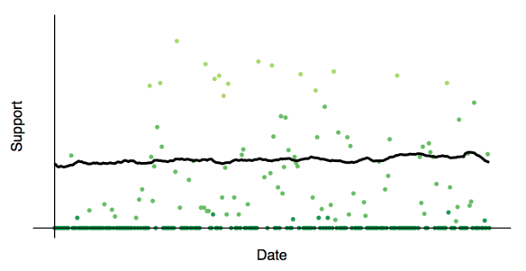
A time-series behavior for one of the items can now be visualized as seen in Figure 2 and using the same convention (green – low support requirement, red – high support requirement). The black line represents the baseline support requirement (note the fluctuation in baseline support, as it is calculated on a weekly basis) for peers with similar configuration.
By using this population-based insight into the behavior of the install base, EMC as well as other manufacturers faced with similar challenges can model, estimate and quantify a baseline level of support for custom tailored manufactured products. They can use the time-series behavior of each of these items; identify the over-demanding ones and act to maintain conformity with the baseline when needed. This approach fundamentally transitions service mode from reactive to proactive, saving operational costs while improving customer experience.
